Deforestation study using GRASS GIS

1   Introduction

We want to study deforestation in the state of Georgia. We will use the National Land Cover Database (NLCD) provided by the Multi-Resolution Land Characteristics (MRLC) Consortium. Our objective is to

1. Calculate the average annual deforestation rate overall (%/year) and per capita (mi<sp>2</sp>/year/capita) for all the counties in Georgia from 2001 and 2016.
2. Find which county has lost the most forest overall (%/year) and per capita (mi<sp>2</sp>/year/capita).
3. Find which county has lost the least or gained the most forest overall (%/year) and per capita (mi<sp>2</sp>/year/capita).
4. Finally, report the statewide annual average deforestation rate per capita and how many and percentage of counties are worse than the statewide average per capita.

2   Data

We can download the following land cover data sets:

• NLCD 2001 Land Cover (CONUS)
• NLCD 2016 Land Cover (CONUS)
• Counties Georgia

3   XY location

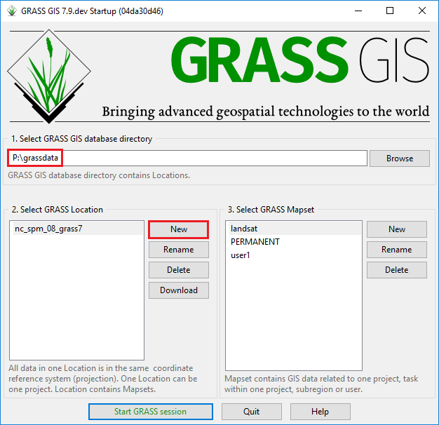
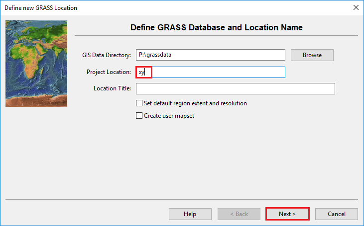
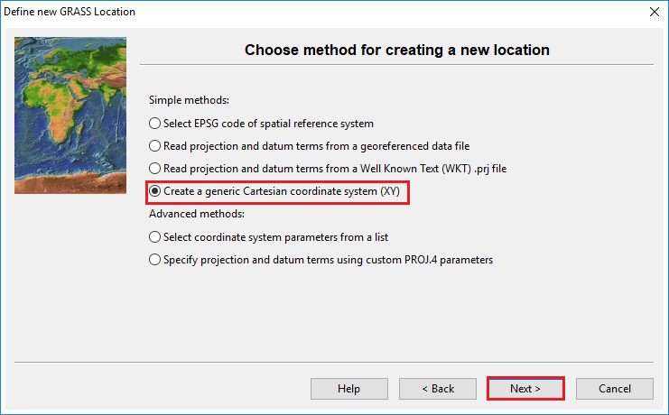
Remember that locations in GRASS can only have one projection. However, it is very rare that different data products we download from different providers are all in the same projection. What it means is that we most likely need to create multiple locations even for the same study. It can be sometimes very challenging to deal with different projections in GRASS because we have to know the projection of each data product we try to import. Without this information, we just cannot create a new location for the data. We can use some external utilities to figure out data projections, but GRASS also provides useful modules. To use these GRASS modules, we have to execute GRASS first obviously, but in what projection? The most basic and simplest projection in GRASS is the XY projection, which is not really any projection at all. This projection does not perform any coordinate transforms when importing/exporting data. However, we can use a location in the XY projection to access GRASS modules.

Now, start GRASS in the new xy location.

4   Figuring out the projection of NLCD data sets

Any data providers should provide metadata about their data. NLCD data sets also come with XML metadata files. For example, for the 2001 NLCD data, we can find NLCD_2001_Land_Cover_L48.xml. The <spref> tag in this metadata file is what we need. NLCD uses its own custom projection. This search will give a list of spatial references that mention NLCD. All these spatial references use the Geodetic Reference System 1980 (GRS80) ellipsoid, but I found that NLCD has recently (not sure when) changed the ellipsoid from GRS80 to the World Geodetic System 1984 (WGS84). These two ellipsoids are almost identical, but they are different. To import NLCD data, we need to create a new location in the Albers Conical Equal Area projection with the WGS84 ellipsoid. There are some more details in the metadata file. We have two options: (1) manually construct projection parameters for GRASS or (2) use a GRASS module to create a new location in the NLCD projection. Which method do I prefer? Well... option (2) of course unless I know I already have a location in the same projection.

There are three important modules in GRASS that can import raster data:

• r.in.gdal: Imports raster data into the current or a new location
• r.import: Imports and reprojects raster data on the fly into the current location
• r.external: Links external raster data sources as a pseudo raster map

Since the NLCD data sets we downloaded are huge (40 GB uncompressed), we just want to create links to these files using r.external and extract the Georgia area later for our study. Both r.in.gdal and r.external provide the -j flag that checks the projection and exits. However, only r.in.gdal can create a new location using the -c flag and the projection information. We’ll check the projection first.

r.in.gdal -j input=NLCD_2001_Land_Cover_L48_20190424.img
WARNING: Projection of dataset does not appear to match current location.

         Dataset PROJ_INFO is:
         name: Albers_Conical_Equal_Area
         datum: wgs84
         ellps: wgs84
         proj: aea
         lat_1: 29.5
         lat_2: 45.5
         lat_0: 23
         lon_0: -96
         x_0: 0
         y_0: 0
         towgs84: 0,0,0,-0,-0,-0,0
         no_defs: defined

         ERROR: proj

5   Creating a new location for NLCD data sets

We can create a new location using r.in.gdal. Since creating a new location won’t import any data, the output parameter’s value doesn’t matter.

r.in.gdal -c input=NLCD_2001_Land_Cover_L48_20190424.img output=dummy location=aea-nlcd-wgs84

Note that we try to use an informative location name “aea-nlcd-wgs84” in the command above because some old NLCD data sets may be in GRS80.

6   Importing the projection of the Georgia counties shapefile

Similarly, GRASS has three vector modules that we can use to import vector data:

• v.in.ogr
• v.import
• v.external

Let’s check the projection of Counties_Georgia.shp.

v.in.ogr -j Counties_Georgia.shp
WARNING: Projection of dataset does not appear to match current location.

         Dataset PROJ_INFO is:
         name: WGS 84
         datum: wgs84
         ellps: wgs84
         proj: ll
         no_defs: defined

         ERROR: proj

Based on the proj parameter, we know that this projection is unprojected and is in lat/long in the WGS84 datum and ellipsoid. This projection is EPSG:4326, so we’ll create a new location in EPSG:4326 and import the shapefile into the new location.

v.in.ogr input=Counties_Georgia.shp output=ga_counties location=epsg4326-latlong

Since v.in.ogr uses the input name for output by default, we don’t need to specify the output parameter. Again, we used an informative location name “epsg4326-latlong” instead of just “latlong” or “epsg4326.”

7   Linking NLCD data sets

Now, we need to link the NLCD data sets as pseudo GRASS raster maps. For this, we need to exit the xy location and start GRASS again in the aea-nlcd-wgs84 location. Once we’re in this location, we can link the external data sources.

r.external -e input=NLCD_2001_Land_Cover_L48_20190424.img output=nlcd2001
r.external -e input=NLCD_2016_Land_Cover_L48_20190424.img output=nlcd2016

We used the -e flag to extend the extent of the location to each data set.

8   Importing the Georgia vector map

We need to import the Georgia counties map into the aea-nlcd-wgs84 location where we’ll perform most of our analysis.

v.proj location=epsg4326-latlong input=ga_counties

9   Extracting NLCD data sets for the state of Georgia

The CONUS NLCD data sets cover the entire Continental United States (CONUS), but our area of interest is only Georgia. We want to extract only this area to make further analysis more efficient. We can use r.mask and r.mapcalc.

r.mask vector=ga_counties
r.mapcalc expression=ga_nlcd2001=nlcd2001
r.mapcalc expression=ga_nlcd2016=nlcd2016

10   Creating a user mapset

We have imported all the raster and vector maps that we need for our study into the same location that can be used for any other projects as well. Now, we want to isolate these “clean” maps from other maps that we’ll create later for our analysis. This way of map organization is just my personal preference to separate out “project-specific” data from “global” data. You can name this new mapset in any way you want. By default, GRASS will suggest your user name. You may use the study name “ga-deforestation.” Create your own mapset and restart GRASS in that mapset.

11   Reclassifying NLCD data sets

NLCD data sets have many classes (2001 and 2016), but we’re only interested in forest area. There are three forest classes including 41, 42, and 43, but, in general, we can say any 40s classes are forest. We can either extract these classes as 1 and the other classes as 0 using r.mapcalc, or reclassify them using r.reclass. In most cases, reclassifying will be much faster than performing map algebra, so we want to use r.reclass. First, let’s reclassify the 2001 land cover map. This module expects a rule file, but we’ll just type in the console (a special filename -). The “*” symbol means the rest of cell values, so we don’t want to use it in the first line.

r.reclass input=ga_nlcd2001 output=ga_forest2001 rules=-
Enter rule(s), "end" when done, "help" if you need it
CELL: Data range is 0 to 95
> 40 thru 49 = 1 forest
> * = 0 non-forest
> end

Then, repeat it for the 2016 map.

r.reclass input=ga_nlcd2016 output=ga_forest2016 rules=-
Enter rule(s), "end" when done, "help" if you need it
CELL: Data range is 0 to 95
> 40 thru 49 = 1 forest
> * = 0 non-forest
> end

12   Display the maps together

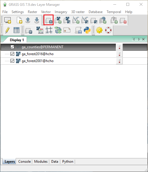
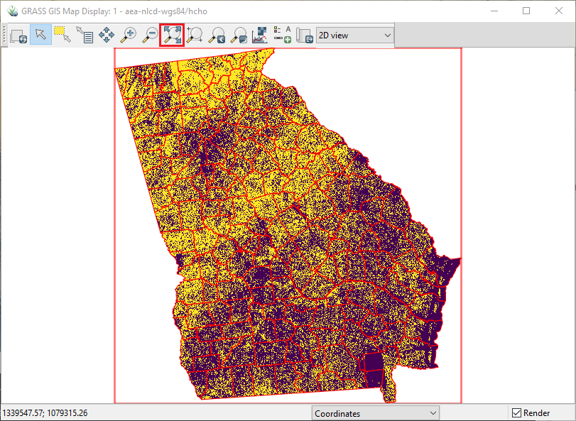
Using the highlighted icon below, we can add multiple maps at once.

Zoom to the study area by selecting ga_counties and clicking the zoom to layer button. Go to the properties window of ga_counties, and change the feature and area fill colors to red and transparent, respectively.