\[ \newcommand\si[1]{\mathrm{#1}} \newcommand\SI[2]{#1\,\si{#2}} \newcommand\matr[1]{\mathbf{#1}} \DeclareMathOperator*{\argmax}{arg\,max} \DeclareMathOperator*{\argmin}{arg\,min} \]
GIS data analysis
1 Data analysis
Decision making process
Answer your research questions
1.1 Questions for GIS analysis
Think about locations, patterns, trends, conditions, implications, etc.
Identify
Queries: Method of data retrieval; We’ve tried these already!
- Select by attributes: Aspatial query (e.g., how many haunted houses in your town?)
- Select by location: Spatial query (e.g., how many houses within 10 miles of your house?)
More complex analyses
1.2 Vector vs. raster
Vector
- Topology
- Complexity
- Computational time
Raster
- Resolution
- Scales of measurement (nominal vs. ratio)
1.3 Data analysis terminology
| Term | Definition |
|---|---|
| Entity | An individual point, line or area in a GIS database |
| Attribute | Data about an entity |
| Feature | An object in the real world to be encoded in a GIS database |
| Data layer | A data set for the area of interest in a GIS |
| Image | A data layer in a raster GIS |
| Cell | An individual pixel in a raster image |
| Function/operation | A data analysis procedure performed by a GIS |
| Algorithm | The computer implementation of a sequence of actions designed to solve a problem |
2 Measurements
Remember! Measurements are only approximations because GIS uses straight line segments (vector) or grid cells (raster).
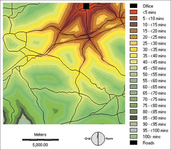
2.1 House hunting case study
Distance from the office calculated using the proximity method
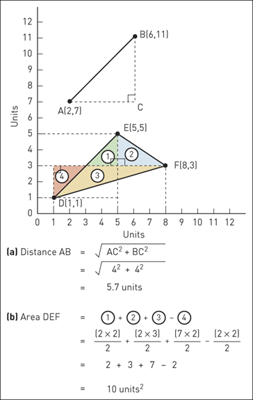
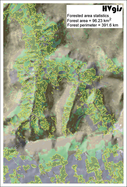
2.2 Calculating lengths and areas
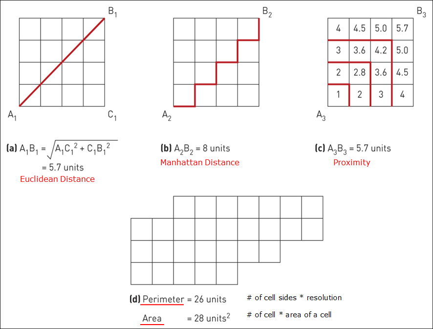
2.3 Different distances
3 Buffering
Creates a zone of interest at a uniform distance around an entity (e.g., within 2 miles)
Many uses
- Identifying entities within a buffer
- Filtering neighbors used in raster
- Can be complex when incorporating slope, accessibility, etc.
3.1 Buffering different geometry types
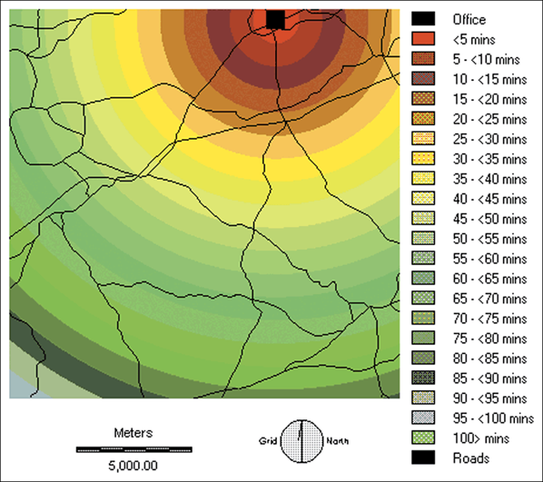
3.2 House hunting case study
Distance from the office adjusted for the road network
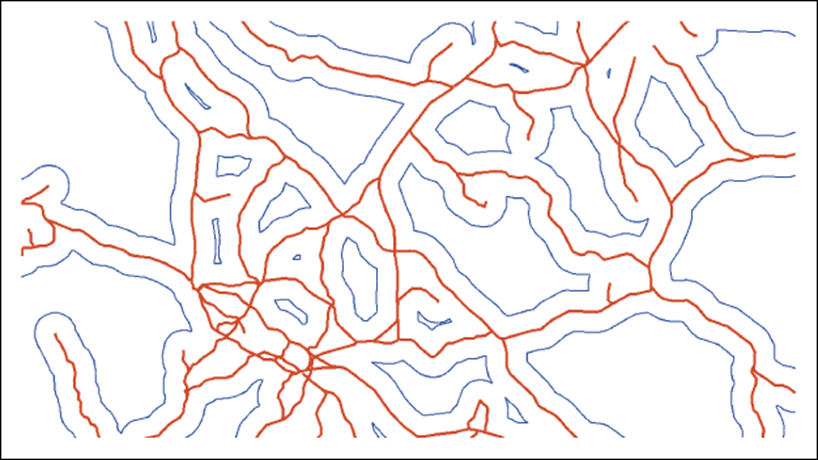
3.3 Radioactive waste case study
Local accessibility of potential disposal sites; 3 km buffer zones (blue) around the rail network (red)
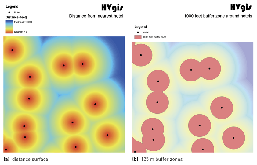
3.4 Proximity map for hotels
4 Spatial interpolation
Procedure for estimating the values at unsampled sites within an area covered by existing observations
Fills in gaps (e.g., height contours)
Inevitable uncertainty with interpolation
Edge effect due to less sampling near edges
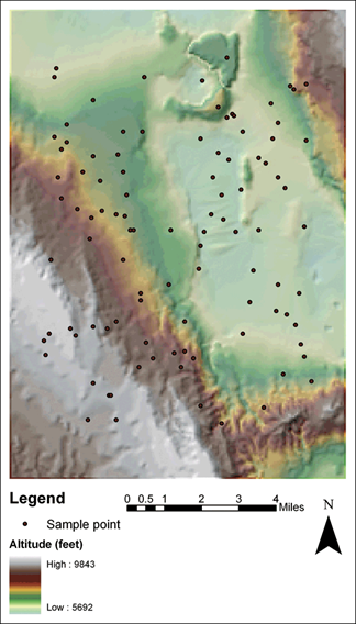
4.1 Original terrain surface with sample points
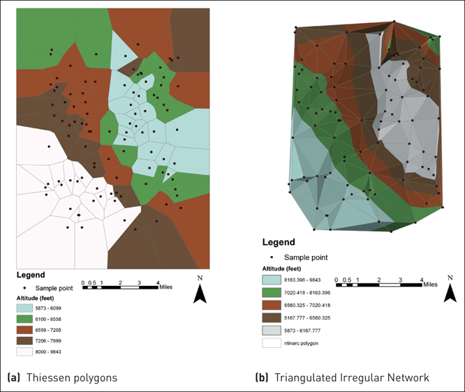
4.2 Interpolation methods
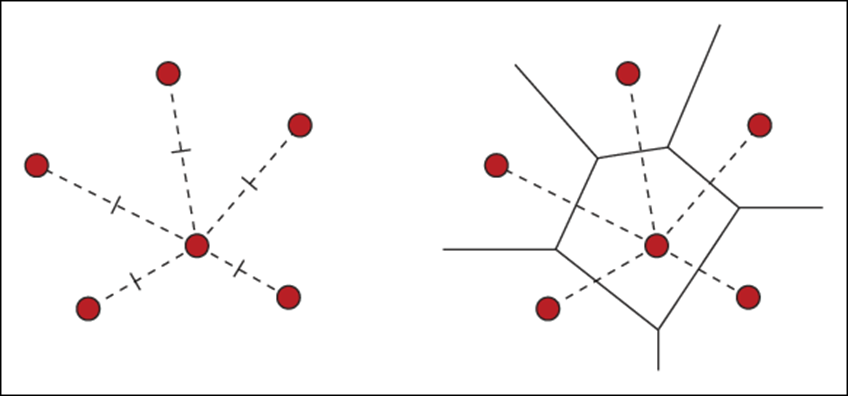
5 Thiessen polygon
Also called the Voronoi diagram.
all locations in the Voronoi polygon are closer to the generator point of that polygon than any other generator point in the Voronoi diagram in Euclidean plane
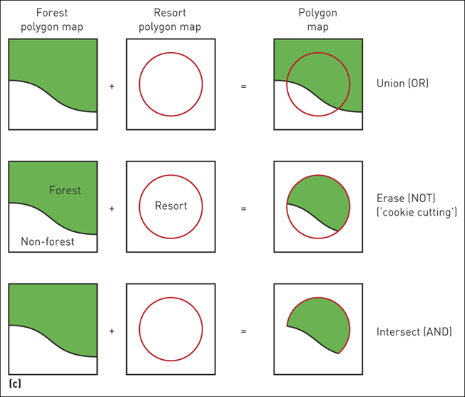
6 Boolean operators
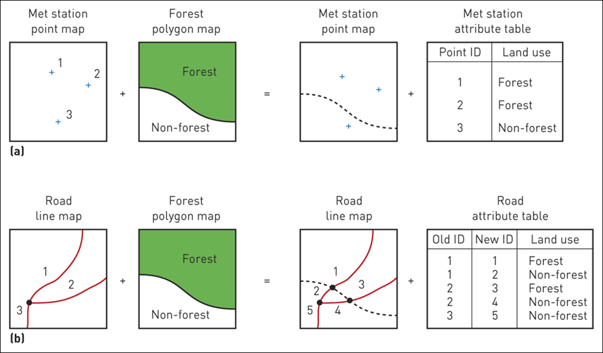
7 Map overlay
One of the key functions
Merges two or more data layers into a new layer
Vector
- Uses geometries (topology)
- Time consuming, complex
Raster
- Map algebra
- Add, subtract, multiple, or divide overlain pixels to produce output pixels
- Quick, efficient, straightforward
7.1 Vector overlays
(a) Point in polygon; (b) Line in polygon; (c) Polygon on polygon
7.2 Raster overlays
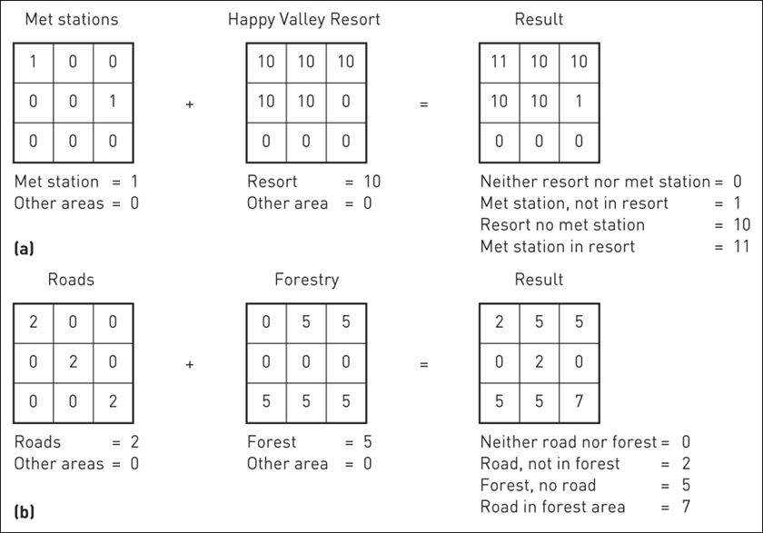
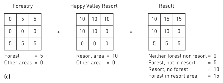
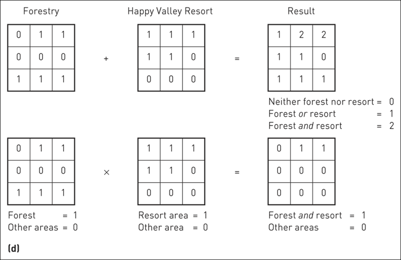
(a) Point in polygon (using add); (b) Line in polygon (using add); (c) Polygon on polygon (using add); (d) Polygon on polygon (using boolean alternatives)
8 Reclassification
Reassigns pixel values in raster to simplify the raster.
For example, cells with values = forestry (value 10) should take a new value of 1.
Cells with values not equal to forestry should take a new value of 0.
Creates a newly coded simple raster.
9 Zonal statistics
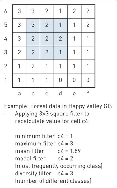
Raster GIS filter operations
9.1 Moving average
(a) Moving average in vector; (b) Moving average in raster
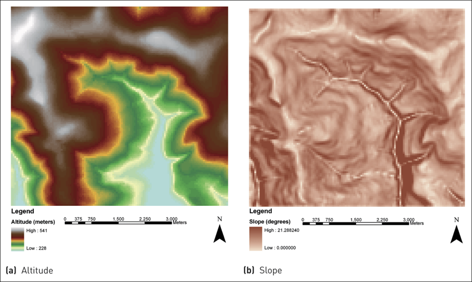
10 Slope
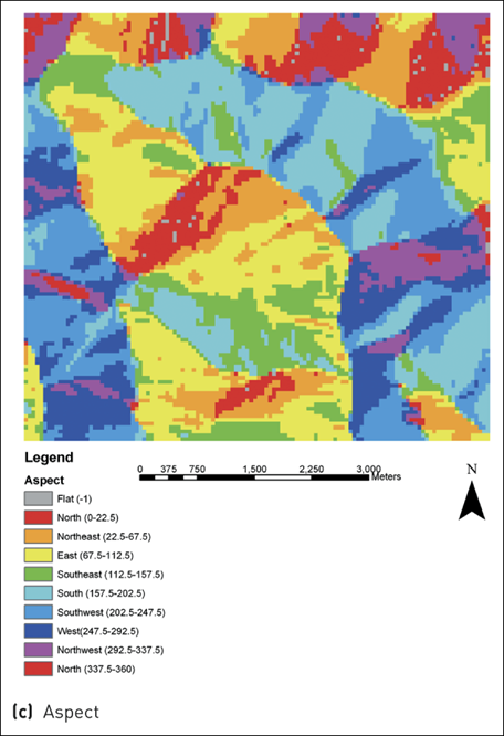
11 Aspect
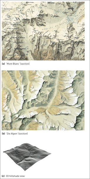
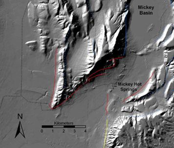
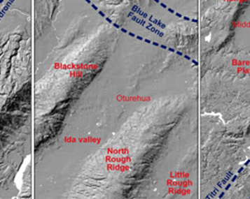
12 Hillshade
Example of cartographic hillshading techniques
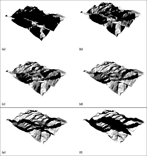
13 Solar radiation
Modelling incoming solar radiation in Happy Valley (a–d) representing morning to evening during a winter’s day
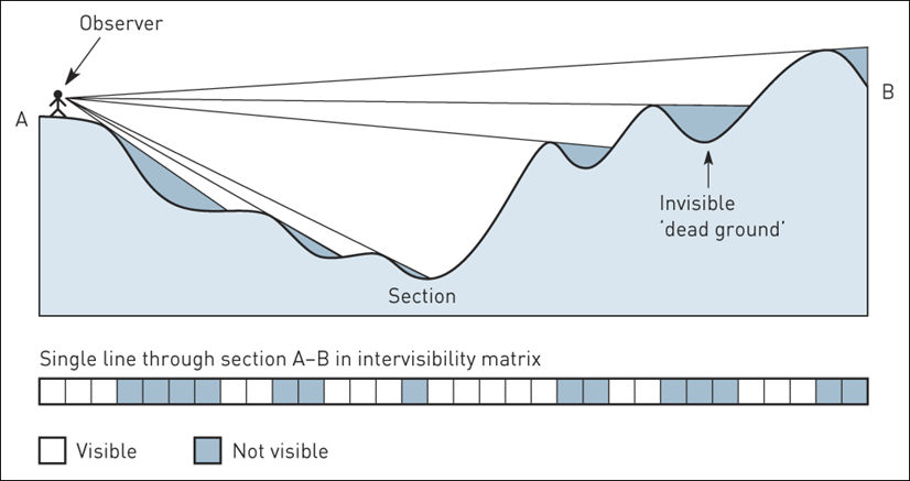
14 Line of sight
Ray tracing for visibility analysis
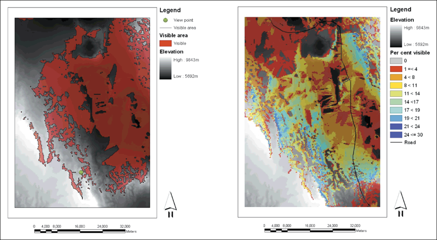
15 Viewshed
Results of viewshed analyses for single point and linear feature
